Reprojecting the Perseverance landing footage onto satellite imagery

Introduction

The landing of the Mars 2020 Perseverance rover last month amazed the world. The stunning footage of the descent shows each stage of the sequence. If you have not seen it already you can watch it here.

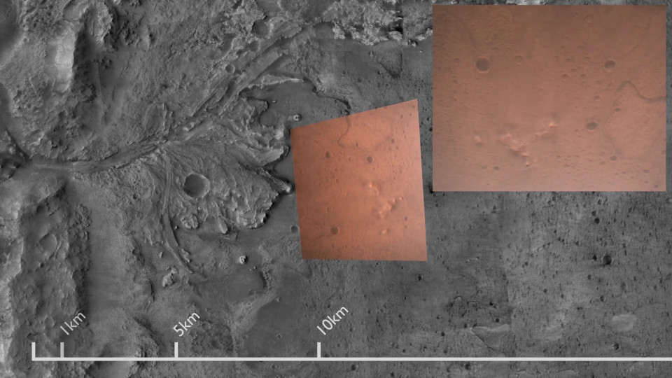
One thing that I found remarkable was the self-similarity of the martian terrain. As the lander descends towards the ground it is hard to get a sense of scale, since there is no familiar frame of reference to tell us how far away the ground is. This led me to embark on a project in which I reproject the footage onto a satellite image obtained from the Mars Express Orbiter, along with a scale to tell us how large features on the ground actually are:

In this post I am going to explain how I used Python, OpenCV, PyTorch, and Blender to make the above footage.

Keypoints and correspondences

Producing my video involves distorting the frames of the original footage so that each frame lines up with the satellite image. The usual way of doing this is to:

• produce some salient keypoints from each image
• find correspondences between the points
• find a mathematical function that maps points in the first image to those in the second image.

The details of implementing the above are described in this OpenCV tutorial, but I will summarize the process here.

Breaking this down, on the left is a frame from the video that we wish to align, with the reference satellite image on the right:

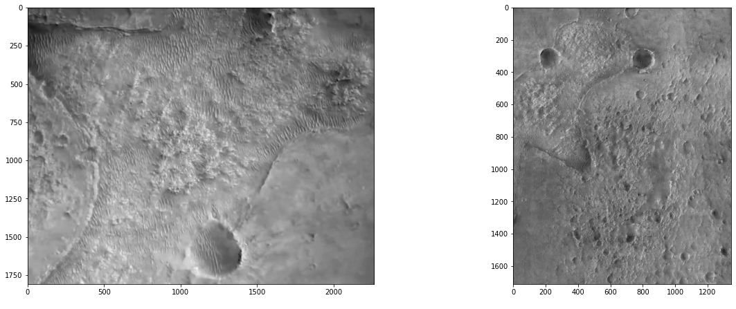
Firstly, we use OpenCV’s Scale Invariant Feature Transform (SIFT) keypoint detector to pull out salient keypoints from the image:

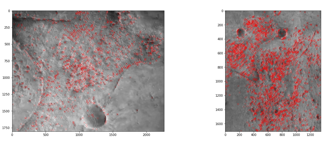
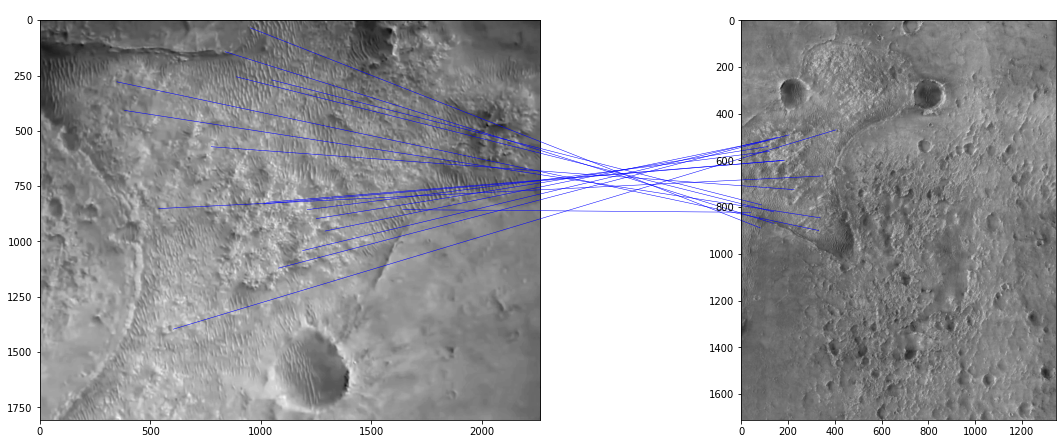
Each red cross here marks a potentially “interesting” point as determined by the SIFT algorithm. Associated with each point (but not shown) is a vector of 128 values which describes the part of the image that surrounds the keypoint. The idea is that this descriptor is invariant to things like scale (as the name implies), rotation, and lighting differences. We can then match up points in our pair of images with similar descriptors:

Projective transformations

Now that we have found the keypoint pairs, the next step is to find a transformation that maps the keypoints from the video frame onto the corresponding keypoints of the satellite image. To do this, we make use of a class of transformations known as projective transformations. Projective transformations can be used to describe how fixed points on a flat plane change apparent position when viewed from a different location and angle, which is useful to us since the surface of Mars can be well approximated by a flat plane at these distances. This is assuming that the camera conforms to a rectilinear perspective projection (i.e. without lens distortion), which appears to be the case.

A projective transformation is represented by a 3x3 matrix \(M\). To apply such a transformation to a 2D point \(v\) we first append a 1 to give a 3-vector, then multiply by the matrix:

To get back to a 2D point, the result is divided by its third element, and truncated back to a 2-vector:

This can be visualized by plotting the points on the z=1 plane, applying the transformation, and then projecting each point towards the origin, back onto the z=1 plane:

When we talk about composing projective transformations, what we are actually doing is multiplying the underlying matrices: projective transformations have the property that the composition of two transformations is equal to the projective transformation given by the matrix product of their respective matrices. Written symbolically this can be written as

where \(p_{M}\) denotes the projective transformation associated with the 3x3 matrix \(M\).

Finding the transformation is done using a RANSAC approach. For more details on RANSAC please see my Pluto flyby post.

Once we have a transformation for each frame, we can reproject each video frame into the frame of reference of the satellite image, thus obtaining the stablized view.

Finding transformations for each frame

Unfortunately it is not simply a case of repeating the above process for each frame in order to produce a complete video, because the algorithm is not able to produce sufficient correspondences for every frame.

In order to resolve this, we also look for transformations between the video frames themselves. The idea being that if a frame has no direct transformation linking it to a satellite image, but we do have a transformation linking it to another frame that is itself connected to the satellite image, then we can simply compose the two transformations to map the original frame onto the satellite view.

So, I labelled every thirtieth frame (ie. one frame per second) as a “keyframe”, and then exhaustively searched for transformations between each pair of keyframes. For the remaining frames I searched for transformations to the nearest keyframe.

This results in a fairly dense graph with one node per frame, and one edge per transformation found. Here is a simplified example, with keyframes at every 5 frames rather than at every 30:

Any path from the satellite node to a particular frame’s node represents a chain of transformations that when composed will map the frame onto the satellite view.

We will begin by selecting one path for each node. Doing a breadth-first search from the satellite node will give us a path to each frame while also guaranteeing that it is the shortest possible:

We want the shortest path possible, because small errors accumulate with each extra transformation.

Here is a short clip made using shortest path transformations:

Optimization

While the above method yields a decent reprojection, it is not perfect. There are clear mode switches around when the shortest path changes.

If we incorporate all correspondences, and not just those on the shortest path, this provides more information and results in smoother and more accurate transformations.

To do this, I wrote a loss function which returns the total reprojection error, given a satellite-relative transformation for each image:

def project(v):
    # Project onto the plane z=1
    return v / v[..., -1][..., None]

def loss(frame_transforms, src_pts, dst_pts, src_idx, dst_idx):
    M_src_inv = torch.inverse(frame_transforms)[src_idx]
    M_dst = frame_transforms[dst_idx]
    ref_pts = torch.einsum('nij,nj->ni', M_src_inv, src_pts)
    reprojected_dst_pts = project(torch.einsum('nij,nj->ni', M_dst, ref_pts))

    return torch.dist(reprojected_dst_pts, dst_pts)

src_pts and dst_pts are both N x 3 arrays, representing every pair of points in the dataset. frame_transforms is an M x 3 x 3 array representing the candidate transformations, M being the number of frames in the video. frame_transforms are relative to the satellite image, which is to say a point in the satellite image when transformed with frame_transforms[i] should give the corresponding point in frame i.

Since there are multiple point-pairs per frame, src_idx and dst_idx are used to map each half of each point-pair to the corresponding video frame.

The loss function proceeds by taking the first points from each pair, mapping them back into the satellite image’s frame of reference, then mapping them into the frame of reference of the second image. With accurate frame transformations and perfect correspondences, these transformed points should be very close to the corresponding set of second points. The final line of the loss function then measures the Euclidean distance (sum of squares) between the reprojected first points and the (unmodified) second points. The idea is that if we find a set of frame_transforms with a lower loss, then we will have a more accurate set of transformations.

loss is written using Torch. Torch is an automatic differentiation framework with functionality for applying gradient descent (amongst other things). As such we can use it to iteratively improve our frame_transforms:

src_pts, dst_pts, src_idx, dst_idx = dataset
frame_transforms = initial_frame_transforms

optim = torch.optim.Adam([frame_transforms], lr=1e-5)
while True:
    optim.zero_grad()
    l = loss(frame_transforms, src_pts, dst_pts, src_idx, dst_idx)
    l.backward()
    optim.step()

dataset is constructed from the set of correspondences, and the initial_frame_transforms are those derived from composing the transformations along the shortest paths.

After running this loop for a while we obtain the final set of transformations for each frame. This produces a more stable set of transformations:

Rendering

To produce the final video I used the 3D modelling and rendering application Blender. I used Blender’s rich Python scripting interface to animate a quad whose corners follow the reprojected video’s corners. To get the right texture for the quad I took advantage of Blender’s shader system:

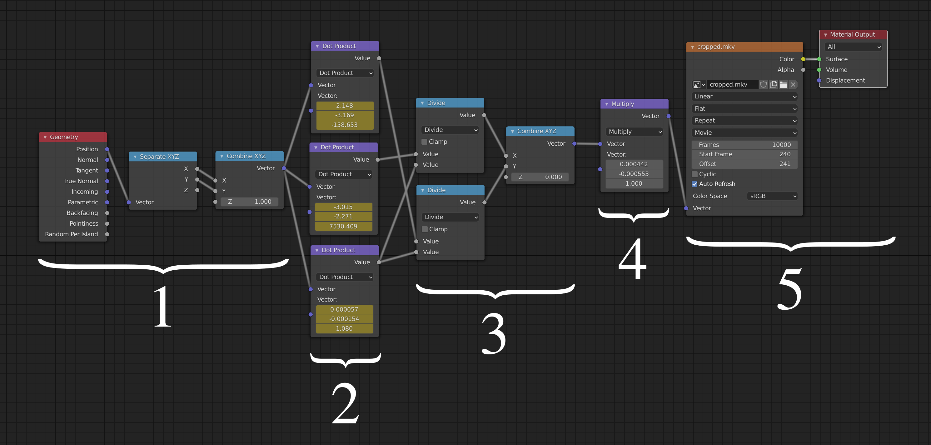
In general, the shader system decides how a particular point on a surface should be shaded, which is typically a function of incoming light, view direction, and properties of the surface. Here I am using it in a very simple way which calculates what colour the point on the quad should be, given the point’s coordinates in 3D space.

Here is a breakdown of the various stages:

1. Take the location of the point to be coloured, and replace the Z component with a 1. This is the first stage of the projective transformation where we turn the 2-vector into a 3-vector by appending a one.
2. Multiply this 3-vector by a matrix defined by the constants shown here. These constants are in fact animated so that on any given frame these display frame_transforms[frame_num].
3. Divide through by z (project onto the z=1 plane).
4. At this point the coordinates are in terms of pixels in the video frame. However the next stage needs them to be in the range 0 to 1, so divide by the video width and height here.
5. Look up the given coordinates in the video, and output the corresponding colour.

Final touches

There are a few extra points that needed addressing to produce the final video:

• I used many satellite images rather than just one. However, I designate one as the “reference frame” (ie. the frame with the identity transformation) and treat the rest as if they were video key frames.
• During the early part of the video, the rover’s heatshield is visible. Without intervention, some frame correspondences track the heatshield (which is itself moving) rather than the terrain, causing bad tracking. So, I manually extracted some keypoints from the heatshield on a particular frame, and ignored all keypoints that were similar to at least one of the heatsheid’s keypoints.
• Rarely, degenerate frame correspondences are found. When all matching keypoints are in a line you get multiple solutions corresponding to rotations about that line. Even if matching keypoints are not exactly in a line but are close, the transformation found can be inaccurate. There was one such image pair that caused this issue in my video, which I manually excluded.

Conclusion

I have shown that the footage from the Perseverance rover’s descent can be stablized and aligned with a reference satellite image. While I am pleased with the result and it certainly helps give context to the raw footage, there are some ways that it could be improved, for example, during the early part of the video there are not many keypoints found by SIFT. This manifests itself as inaccuracy in the tracking. Perhaps experimenting with different keypoint algorithms would yield more usable keypoints.

There may be also alternative ways to solve the problem which I have not explored here. For example, the problem is quite similar to that of general video stabilization. Perhaps I could use an off-the-shelf solver to achieve a similar effect.