12 years in 15 seconds: Aligning and condensing a self-portrait time-lapse

The above is derived from the images in this timelapse video by Noah Kalina (not me!). Used with permission.

Introduction

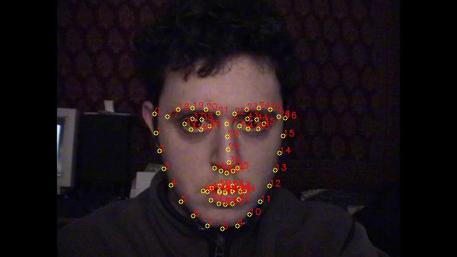
Following from my previous experiments with face alignment, I got to thinking if the same techniques could be applied to photo-a-day time lapse projects, such as Noah Kalina’s 12.5 year (and counting) epic.

The idea is to account for incidental variances to acheive a smooth, yet extremely fast-forwarded view of the subject. Specifically, the variances being eliminated are:

• Face position: The orientation of the face within the frame.
• Lighting: Differences in illumination colour and/or white balance.
• Pose: Differences in facial pose, and lighting direction.

As usual, I’m attacking this problem in Python. The code is relatively short (~250 lines), although I’m using dlib, OpenCV and numpy to do the heavy lifting. Source code is available here.

Aligning

As a first step, lets account for facial position by rotating, translating and scaling images to match the first. Here’s the code to do that:

input_fnames = # Video frames
ref_landmarks = None
for fname in input_fnames:
    im = cv2.imread(fname)

    # Compute landmark features for the face in the image.
    try:
        landmarks = get_landmarks(im)
    except NoFaces:
        print "Warning: No faces in image {}".format(fname)
        continue
    except TooManyFaces:
        print "Warning: Too many faces in image {}".format(fname)
        continue

    # If this is the first image, make it the reference.
    if ref_landmarks is None:  
        ref_landmarks = landmarks

    # Compute the transformation required to map the facial landmarks of the
    # current image onto the reference landmarks.
    M = orthogonal_procrustes(ref_landmarks, landmarks)

    # Translate/rotate/scale the image to fit over the reference image.
    warped = warp_im(im, M, im.shape)

    # Write the file to disk.
    cv2.imwrite(os.path.join(OUT_PATH, fname), warped)

Here, the get_landmarks() function uses dlib to use facial landmark features:

…and orthogonal_procrustes() generates a transformation matrix which maps one set of landmarks features onto another. This transformation is used by warp_im() to translate, rotate and scale images to line up with the first image. For more details refer to my Switching Eds post which uses an identical approach in steps 1 and 2 to align the images.

After correcting for face position, you get a video that looks like this:

Colour adjustment

There are still a few obvious discontinuities. One variance we can easily iron out is the overall change in colour on the face due to different lighting and/or white balance settings.

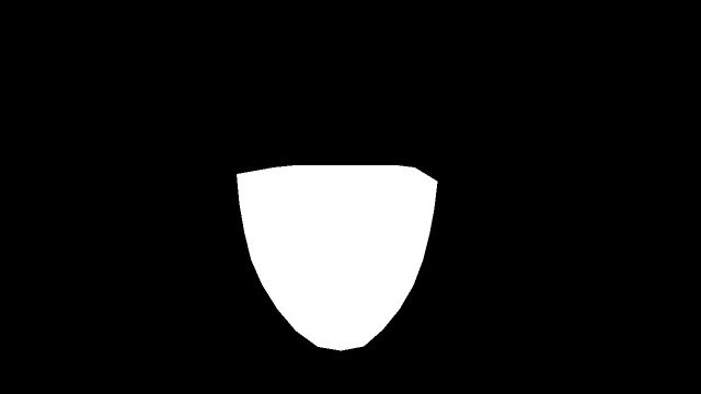
The correction works by computing a mask for each image:

mask = numpy.zeros(im.shape[:2], dtype=numpy.float64)
cv2.fillConvexPoly(mask, cv2.convexHull(points), color=color)

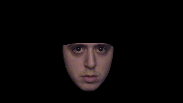
…based on the convex hull of the landmark points. This is then multiplied by the image itself:

masked_im = mask[:, :, numpy.newaxis] * im

The sum of the pixels in the masked image is then divided by the sum of the values in the mask, to give an average colour for the face:

color = ((numpy.sum(masked_im, axis=(0, 1)) /
          numpy.sum(mask, axis=(0, 1))))

Images’ RGB values are then scaled such that their average face colour matches that of the average face colour of the first image:

im = im * ref_color / color

…where ref_color is the color of the first face, saved from the first iteration.

Here’s the first 5 seconds with color correction applied:

Speeding up

The above is looking pretty good, but there are still some issues causing lack of smoothness:

• Minor variations in facial pose.
• Changes in lighting direction.

Given these perturbations are more or less random for each frame, the best we can do is select a subset of frames which is in some sense smooth.

To solve this I went the graph theory route:

Here I’ve split the video into 10 frame layers, with full connections from each layer to the next. The weights of each edge measures how different the two frames are, with the goal being to find the shortest path from Start to End; frames on the selected path are used in the output video. By doing this the total “frame difference” is minimized. Because the path length is fixed by the graph structure, this is equivalent to minimizing the average frame difference.

The metric used for frame difference is the euclidean norm between the pair of images, after being masked to the face area. Here’s the code to calculate weights, a dict of dicts where weight[n1][n2] gives the weight of the edge between node n1 and n2:

names = # Input image names
mask = # Mask which covers the face region
FRAME_SKIP = 10

def find_weights():
    weights = collections.defaultdict(dict) 
    prev_layer = None
    layer = []

    def link_layers(layer1, layer2):
        for name1, im1 in layer1:
            for name2, im2 in layer2:
                weights[name1][name2] = numpy.linalg.norm(im2 - im1)

    for n in names:
        im = cv2.imread(n)
        layer.append((n, (im * mask).astype(numpy.float32)))

        if len(layer) == FRAME_SKIP:
            if prev_layer is not None:
                link_layers(prev_layer, layer)
            prev_layer = layer
            layer = []

    if layer:
        link_layers(prev_layer, layer)

    return weights
weights = find_weights()

And because the graph is in fact a directed acyclic graph we can use a simplified version of Dijkstra’s Algorithm to find the shortest path:

# Find the nodes in the first and last layer.
starts = names[:FRAME_SKIP]
if len(names) % FRAME_SKIP != 0:
    ends = names[-(len(names) % FRAME_SKIP):]
else:
    ends = names[-FRAME_SKIP:]

# Compute `dist` which gives the minimum distance from any frame to a start
# frame, and `parent` which given a node returns the previous node on the
# shortest path to that node.
dist = {n: (0 if n in starts else None) for n in names}
parent = {}
for u in names:
    for v, weight in weights[u].items():
        if dist[v] is None or dist[v] > dist[u] + weight:
            dist[v] = dist[u] + weight
            parent[v] = u

# Find the end node which has least distance, and step through the shortest
# path until we hit a start node.
def drain_to_source():
    v = min(ends, key=lambda v: dist[v])
    yield v
    while v not in starts:
        v = parent[v]
        yield v

# Reverse to find the shortest path.
shortest_path = reversed(list(drain_to_source))

Which yields the final smoother, although shorter video: