Making faces with Haar cascades and mixed integer linear programming
Introduction
I’ve previously mentioned face detection in my Face swapping post. The face detection step there uses the popular “cascade of Haar-like features” algorithm to get initial bounds for faces in an image.
In this post I describe a script I wrote to invert this face detection algorithm: Instead of taking an image and telling you whether it contains a face, it will generate an image of a face, using nothing more than cascade data.
As always, full source code is available on GitHub.
Haar Cascades
In 2001 Viola and Jones introduced their revolutionary object detection algorithm based on cascades of Haar-like features, enabling for the first time real-time detection of faces (and other objects) in video data.
At its core, the algorithm accepts a small (typically 20x20) image along with some precomputed cascade data (described below), and returns whether or not the object of interest is present there. One can then just apply the core algorithm to the full image in multiple windows, with the windows at various scales and positions, returning any where the core algorithm detected the object:
It is this core algorithm that I’m attempting to invert in this post. But how does it work? Well, it’s based on so called Haar-like features:

Each feature is associated with a threshold to form a so-called weak classifer. If the sum of the pixel values in the black region subtracted from the sum of the pixel values in the white region exceed the threshold then the weak classifier is said to have passed. For example, the weak classifier in the first image is detecting a dark area around the eyes compared to above the cheeks.
Features are all defined with axially aligned rectangles and take one of a few basic forms, as shown above. They are defined on the same small (eg. 20x20) grid as the input image.
Weak classifiers are combined into stages. A stage passes based on which weak classifiers associated with the stage pass; each weak classifier has a weight associated with it, and if the sum of all the passing weak classifiers’ weights exceeds a stage threshold then the stage is said to have passed.
The stages, weak classifiers and associated weights are calculated by running a training algorithm on thousands of positive and negative training images. See the Viola-Jones paper for more details.
If all the stages in the cascade data pass then the algorithm returns that an object has been detected.
This can be written in Python like:
def detect(cascade, im):
    for stage in cascade.stages:
        total = 0
        for classifier in stage.weak_classifiers:
            if numpy.sum(classifier.feature * im) >= classifier.threshold:
                total += classifier.weight
        if total < stage.threshold:
            return False
    return True
The input image im is assumed to already have been resized to the small
cascade size. classifier.feature is an array the same shape as im, with
1s at points corresponding with white areas of the feature, -1s at points
corresponding with black areas of the feature, and 0s elsewhere. Note the
actual algorithm as described by Viola and Jones uses integral images to add up
pixel values, one of the reasons for the algorithm’s fast operation.
The main reason for the multiple stages is efficiency: Typically the first stage will contain only a handful of features, but can reject a large proportion of negative images. There are typically hundreds of features in a particular cascade, and a dozen or more stages.
Mixed integer linear programming
In order to invert the detect function described above, I express the
problem in terms of Mixed integer linear programming, and then apply a MILP solver to the
linear program.
Here’s the detect function described in terms of MILP constraints. First the
constraints to ensure a weak classifer passes, if it is required to. Lets call
these feature constraints:
…and a set of constraints to ensure that each stage passes. Let’s call these stage constraints:
\[\forall k \in [0, {N_{stages}} - 1] \ \colon \ \Bigg( \sum_{j \in {classifiers}_k} {passed}_j * {weight}_j \geq stage\_threshold_k \Bigg)\]Where:
- \({pixel}_i \in [0, 1],\) \(0 \leq i < N_{pixels}\) are the pixel values of the
input image. (Corresponds with
imin the code.) - \({feature}_{j,i} \in \mathbb{R},\) \(0 \leq j < N_{classifiers},\)
\(0 \leq i < N_{pixels}\) are the weight values of the feature associated with
weak classifier \(j\). (Corresponds with
classifier.featurein the code.) - \({threshold}_j\) is the threshold value of weak classifier \(j\).
(
classifier.thresholdin the code.) - \({weight}_j\) is the weight of weak classifier \(j\). (Corresponds
with
classifier.weightin the code.) - \({positive\_classifiers}\) is the set of classifier indices with positive weights, ie. \(\{ j \in [0, N_{classifiers} - 1] : {weight}_j > 0 \}\)
- \({negative\_classifiers}\) is the set of classifier indices with negative weights, ie. \(\{ j \in [0, N_{classifiers} - 1] : {weight}_j < 0 \}\).
- \({passed}_j \in \{0, 1\}\) is a binary indicator variable, corresponding with whether weak classifier \(j\) has passed.
- \(M_{j}\) are numbers chosen to be large enough such that if the term they appear in is non-zero, then the inequality holds true.
- \({classifiers}_k\) is the set of weak classifier indices associated with stage \(k\).
- \(stage\_threshold_k\) is the stage threshold of stage \(k\).
(Corresponds with
stage.thresholdin the code.)
The variables to be sought by the MILP solver are the \({pixel}_i\) and \({passed}_j\) values. The rest of the values are derived from the cascade definition itself.
The main thing to note is the use of \({passed}_j\) as an indicator variable, ie. how its state can turn on or off one of the feature constraints. For example, take \(j \in {positive\_classifiers}\). If a particular solution has \({passed}_j\) as 1, then we better be sure that the feature \(j\) actually exceeds the classifier’s threshold, as it is contributing positively towards the stage constraint passing. In this case the \(M_{j} (1 - {passed}_j)\) term in the relevant feature constraint is zero, ie. the constraint is “on”.
Conversely, for a classifier \(j\) with a negative weight, we only care that the feature doesn’t pass its classifier threshold if \({passed}_j\) is 0.
With this in mind, it’s clear that detect(cascade, im) is True if and only
if there’s a solution to the linear program derived from cascade where the \({pixel}_j\) variables take on the corresponding pixel values in im.
MILPs in Python
I chose to use the docplex module to write the above constraints in Python. With this module constraints can be written in a natural way, which are then dispatched to IBM’s DoCloud Service for solving remotely. Note DoCloud requires registration and is not free, although they offer a free month’s trial which is what I used for this project. I did initially try solving the problem with the free PuLP module, with which I had limited success either due to the underlying solver being less sophisticated or limitations of my machine.
As an example, here’s how the variables are defined:
from docplex.mp.model import Model

model = Model("Inverse haar cascade", docloud_context=docloud_context)

pixel_vars = {(x, y): model.continuous_var(
                name="pixel_{}_{}".format(x, y)
                lb=0., ub=1.0)
                for y in range(cascade.height)
                for x in range(cascade.width)}
passed_vars = [self.binary_var(name="passed_{}".format(idx))
                                       for idx in range(len(cascade.features))]
And an (abridged) snippet which adds the stage constraint:
for stage in cascade.stages:
    model.add_constraint(sum(c.weight * passed_vars[c.feature_idx]
                                        for c in stage.weak_classifiers) >=
                                                               stage.threshold)
The problem is then solved by calling model.solve().
If succesful, the pixel variable values are extracted from the solution, and
converted into an image (a numpy array) which can then be written to disk
using cv2 (or similar).
im = numpy.array([[pixel_vars[x, y].solution_value
                    for x in range(cascade.width)]
                  for y in range(cascade.width)])
cv2.imwrite("out.png", im * 255.)
By default, docplex will just search for a feasible solution. However, one
can set an objective like so:
model.set_objective("max",
    sum((c.weight * passed_vars[c.feature_idx]
            for s in self.cascade.stages
            for c in s.weak_classifiers)))
This objective will try and find the solution which most exceeds the stage constraints. It can take an unreasonably long time to find the true maximum, so we can set a time limit:
model.set_time_limit(60 * 60)This line instructs the solver to stop after an hour and output the best solution found so far (if any).
See the source code for the full details. Note the code there is a little more complex due to supporting tilted features and also because of the format of the cascade data in OpenCV, but the essence is the same.
Results
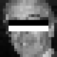
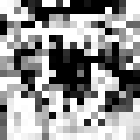
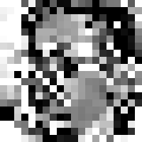
Here’s the output of running the program on OpenCV’s
haarcascade_frontalface_alt.xml cascade for an hour:
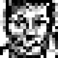
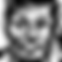
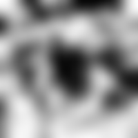
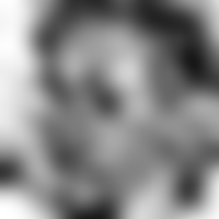
Not bad. Shame about the low resolution, but that’s unavoidable given the features are only defined on a 20x20 grid. Here is the same image blurred, which is more convincingly face-like:
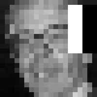
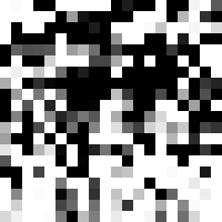
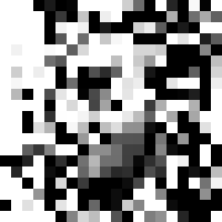
And to test the limits of the detector, lets minimize the stage constraint instead of maximising:
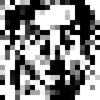
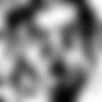
Decidedly less face-like, but should still be detected by OpenCV.
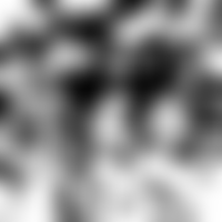
Here’s the best eye image (based on haarcascade_eye.xml)
…and the worst:
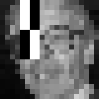
Here’s the best profile face image (based on haarcascade_profileface.xml):
…and the worst:

If you enjoyed this post, please consider supporting my efforts: